flowchart TD

    A([Start Data Ingestion]) --> B[Read Database Configuration]

    B --> C[Connect to PostgreSQL Database]

    C --> D[Load Source Table as DataFrame]

    D --> E[Remove ID Columns]

    E --> F[Replace Missing Values]

    F --> G{Target Column Exists}

    G -- No --> H[Raise Exception]
    G -- Yes --> I[Train Test Split]

    I --> J{Stratify by Target}

    J -- Yes --> K[Stratified Split]
    J -- No --> L[Random Split]

    K --> M[Save Training Data]
    L --> M

    M --> N[Save Testing Data]

    N --> O[Create Data Ingestion Artifact]

    O --> P([End])

1 Overview
Machine learning is a subset of artificial intelligence (AI) that enables systems to learn from data, identify patterns, and make decisions or predictions without being explicitly programmed for every task.
The goal of this project is to predict customer churn using supervised machine learning in order to support proactive retention strategies and improve customer lifetime value.
2 Problem Statement
Customer churn poses a significant challenge for subscription-based and service-oriented businesses, as acquiring new customers is often more costly than retaining existing ones. The objective of this project is to develop a robust machine learning pipeline to predict customer churn, enabling early identification of customers who are likely to discontinue a service. By accurately modeling churn behavior, organizations can implement targeted retention strategies, optimize customer engagement, and reduce revenue loss.
To address this problem, the workflow leverages historical customer data to train and evaluate multiple classification models under a structured and reproducible MLOps framework. The system emphasizes data validation, drift detection, systematic model comparison, overfitting monitoring, and experiment tracking, ensuring that the selected model generalizes well to unseen data and is suitable for deployment in a production inference environment.
3 System Overview
This project is designed as a production-oriented machine learning system, organized into the following satges:
4 Data Ingestion
The Data Ingestion stage used in the pipeline extracts data from a PostgreSQL source, performs basic cleaning and validation, splits the data into training and testing sets, and saves the resulting artifacts for downstream stages.
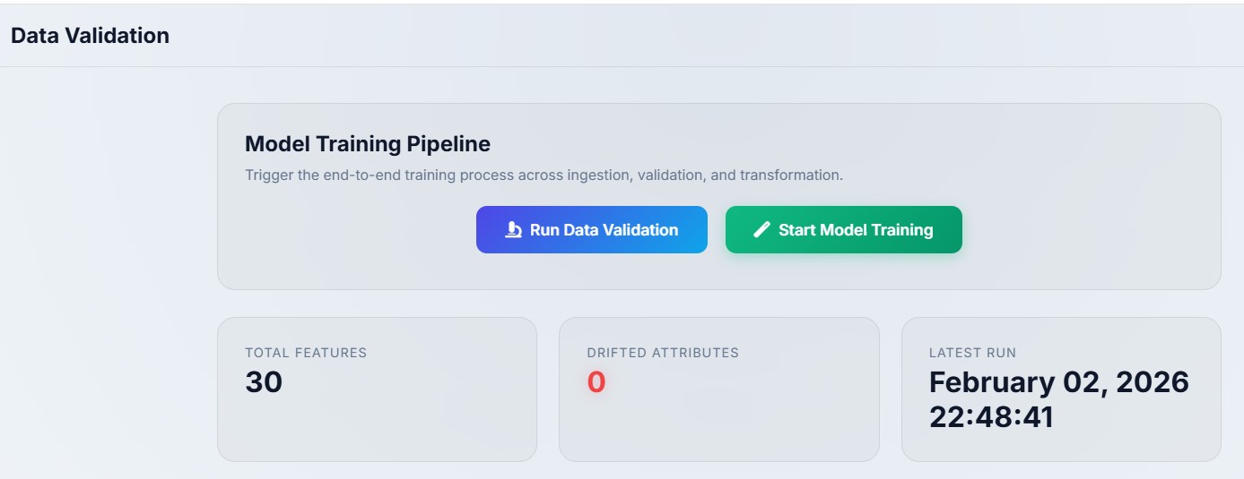
5 Data Validation
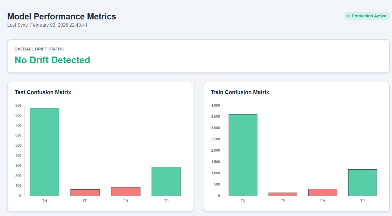
The Data Validation stage ensures the reliability and consistency of data before model training. It begins by validating schema conformity and confirming the presence of the target variable, preventing structural issues from propagating downstream. To evaluate data stability, the pipeline performs statistical drift detection between training and testing datasets using the Kolmogorov–Smirnov (KS) test for numerical features and the Chi-square test for categorical features.
For the KS test, the null hypothesis (H₀) states that the training and testing samples are drawn from the same underlying distribution, while the alternative hypothesis (H₁) indicates a distributional shift. The test compares the empirical cumulative distribution functions (CDFs) of the two samples and computes the maximum absolute distance between them:
\[ D = \sup_x \left| F_{\text{train}}(x) - F_{\text{test}}(x) \right| \]
A feature is flagged for drift if the p-value < 0.05, indicating that the observed CDF difference is unlikely to be due to random sampling.
For the Chi-square test, H₀ assumes that categorical feature frequencies remain consistent across datasets, while H₁ suggests a significant change in distribution. Drift is quantified by comparing observed and expected category counts using:
\[ \chi^2 = \sum_{i=1}^{k} \frac{(O_i - E_i)^2}{E_i} \]
where \(( O_i )\) represents the observed frequency of category \(( i )\), \(( E_i )\) is the expected frequency derived from the training distribution, and \(( k )\) is the number of categories. A categorical feature is flagged for drift when the p-value < 0.05, signaling a statistically significant change in category proportions. Based on these decision rules, a drift report is generated and validation artifacts are produced to support traceability and downstream pipeline decisions. The workflow below summarises the Data Validation stage.
flowchart TD

    A([Start Data Validation])

    A --> B[Load Schema from YAML]

    B --> C[Load Train and Test CSV Files]

    C --> D[Validate Column Structure<br/>Against Schema]

    D -->|Mismatch| E[Save Data to Invalid Paths]
    E --> F[Write Error Report]
    F --> G[Create DataValidationArtifact<br/>Status = Failed]
    G --> H([End])

    D -->|Valid| I[Validate Target Column Presence]

    I -->|Missing| E

    I -->|Present| J[Detect Dataset Drift]

    J --> K[KS Test for Numerical Columns]
    J --> L[Chi-Square Test for Categorical Columns]

    K --> M[Generate Drift Report YAML]
    L --> M

    M --> N[Save Valid Train and Test Data]

    N --> O[Create DataValidationArtifact<br/>Status = Success]

    O --> P([End])
6 Data Transformation
Validated datasets are filtered, encoded, and preprocessed using dedicated pipelines for numerical and categorical features. The transformed datasets and preprocessing object are saved as artifacts for downstream model training, as summarised in the following workflow.
flowchart TD

    A([Start Data Transformation])

    A --> B[Load Valid Train and Test Data]

    B --> C{Target Column Exists}

    C -- No --> D[Raise Exception]
    C -- Yes --> E[Filter Allowed Target Classes]

    E --> F[Separate Features and Target]

    F --> G[Encode Target Labels]

    G --> H[Identify Numeric and Categorical Columns]

    H --> I[Build Preprocessing Pipeline]

    I --> J[Fit and Transform Training Features]

    J --> K[Transform Testing Features]

    K --> L[Combine Transformed Features and Target]

    L --> M[Save Transformed Train and Test Arrays]

    M --> N[Save Preprocessing Object]

    N --> O[Create DataTransformationArtifact]

    O --> P([End])
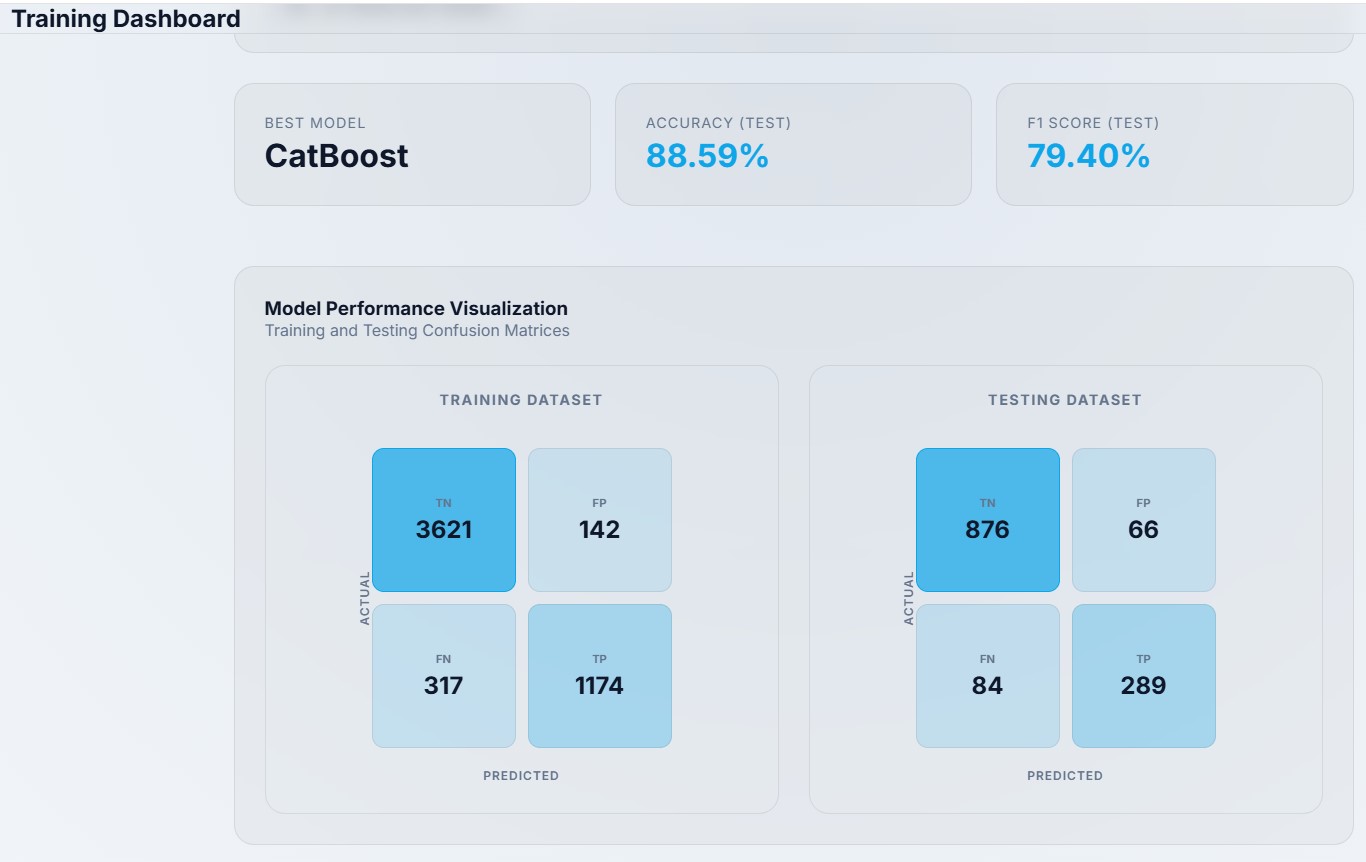
7 Model Training
The Model Training stage adopts a comparative approach in which multiple classification algorithms are trained and evaluated to identify the best-performing model. Rather than relying on a single estimator, the workflow includes models with different inductive biases to capture linear relationships, non-linear patterns, distance-based structures, and complex feature interactions.
- Linear models (Logistic Regression, SGD Classifier): provide strong, interpretable baselines and perform well when the decision boundary is approximately linear.
- Distance-based models (K-Nearest Neighbors): capture local neighborhood patterns and non-parametric relationships in the feature space.
- Margin-based models (Support Vector Machines): are effective in high-dimensional spaces by maximizing class separation.
- Probabilistic models (Naive Bayes): offer fast training and serve as simple baselines under conditional independence assumptions.
- Tree-based models (Decision Trees): model non-linear relationships and feature interactions with minimal preprocessing.
- Ensemble tree methods (Random Forest, Gradient Boosting, AdaBoost): improve generalization by aggregating multiple weak learners and reducing variance or bias.
- Gradient boosting frameworks (XGBoost, LightGBM, CatBoost): deliver state-of-the-art performance on structured tabular data through efficient boosting, regularization, and optimized tree construction.
All models are trained using predefined hyperparameter grids and evaluated consistently on training and test datasets using standardized classification metrics. The best-performing model is selected based on empirical performance while monitoring for overfitting, ensuring a balance between predictive accuracy and generalization. The following steps are taken to train and evaluate the models:
7.0.1 Data Preparation
The transformed dataset is split into features and labels:
\[ \mathbf{X}*{train}, \mathbf{y}*{train}, \quad \mathbf{X}*{test}, \mathbf{y}*{test} \]
7.0.2 Model Candidates
Multiple classification models are evaluated:
\[ \mathcal{M} = { \text{Tree-based}, \text{Linear}, \text{Distance-based}, \text{Kernel-based}, \text{Boosting} } \]
7.0.3 Model Selection
Each model is trained and evaluated, and the best model is selected using a performance score:
\[ m^* = \arg\max_{m \in \mathcal{M}} ; \text{Score}(m) \]
7.0.4 Training and Prediction
The selected model is trained and used to generate predictions:
\[ \hat{\mathbf{y}}*{train} = m^*(\mathbf{X}*{train}), \quad \hat{\mathbf{y}}*{test} = m^*(\mathbf{X}*{test}) \]
7.0.5 Evaluation Metrics
Performance is evaluated using standard classification metrics:
\[ \text{Accuracy}, \quad \text{Precision}, \quad \text{Recall}, \quad \text{F1} \]
7.0.6 Overfitting Check
Training and testing accuracy are compared:
\[ \Delta = \left| \text{Accuracy}*{train} - \text{Accuracy}*{test} \right| \]
A warning is raised if ( ) exceeds a predefined threshold.
7.0.7 Model Artifacts
The final outputs saved for deployment are:
\[ { \text{Trained Model}, \text{Preprocessor}, \text{Predictions}, \text{Evaluation Metrics} } \]
7.1 Model Training Workflow
The following flowchart presents a simplified view of the model training pipeline used in this project.
It focuses on the core stages from data preparation to model persistence, abstracting away implementation details.
flowchart TD

    A([Start Model Training]) --> B[Load Pre-split Transformed Data]

    B --> C[Separate Features and Target]

    C --> D[Define Candidate Models]

    D --> E[Train and Evaluate Models]

    E --> F[Select Best Performing Model]

    F --> G[Evaluate on Train and Test Data]

    G --> H{Overfitting Check}

    H -->|Detected| I[Log Warning]
    H -->|Not Detected| J[Proceed]

    I --> J

    J --> K[Log Metrics and Model with MLflow]

    K --> L[Save Model and Artifacts]

    L --> M([End])
8 Deployment
To build reliable and reproducible solutions, model development must follow a structured workflow that supports systematic experimentation, consistent evaluation, and clear traceability. The following workflow outlines a production-aligned model training process that starts from pre-split, transformed data and progresses through candidate model definition, training, evaluation, and selection using a unified and repeatable pipeline.
A key component of the workflow is the overfitting check, where discrepancies between training and test performance are monitored and logged without prematurely interrupting experimentation. All metrics, trained models, and diagnostic artifacts are tracked using MLflow, while finalized models and preprocessing artifacts are packaged and stored in Cloudflare R2 as versioned objects. This separation of development and artifact storage enables a smooth transition to production inference environments, ensuring scalability, auditability, and reliable model deployment.
flowchart TD

    %% ======================
    %% DEVELOPMENT REGION
    %% ======================
    subgraph DEV["Development Phase"]
        A([Start Model Training])
        --> B[Load Pre-split Transformed Data]
        B --> C[Separate Features and Target]
        C --> D[Define Candidate Models]
        D --> E[Train and Evaluate Models]
        E --> F[Select Best Performing Model]
        F --> G[Evaluate on Train and Test Data]
        G --> H{Overfitting Check}
        H -->|Detected| I[Log Warning in MLflow]
        H -->|Not Detected| J[Proceed with Pipeline]
        I --> J
        J --> K[Log Metrics, Params & Model in MLflow]
        K --> L[Package Model & Artifacts]
    end

    %% ======================
    %% CLOUDFLARE R2
    %% ======================
    subgraph R2["Cloudflare R2 (Artifact Storage) Phase"]
        M[Upload Model Artifacts to Cloudflare R2]
        --> N[Versioned Artifact Storage]
    end

    %% ======================
    %% PRODUCTION REGION
    %% ======================
    subgraph PROD["Production Phase"]
        O[Load Model from Cloudflare R2]
        --> P[Initialize Inference Service]
        --> Q[Serve Predictions via API]
        --> R([End - Production Inference])
    end

    %% Cross-region links
    L --> M
    N --> O

    %% ======================
    %% REGION STYLES (KEY FIX)
    %% ======================
    style DEV fill:#f5f5f5,stroke:#d1d5db,stroke-width:2px
    style R2 fill:#f9fafb,stroke:#d1d5db,stroke-width:2px
    style PROD fill:#f5f5f5,stroke:#d1d5db,stroke-width:2px
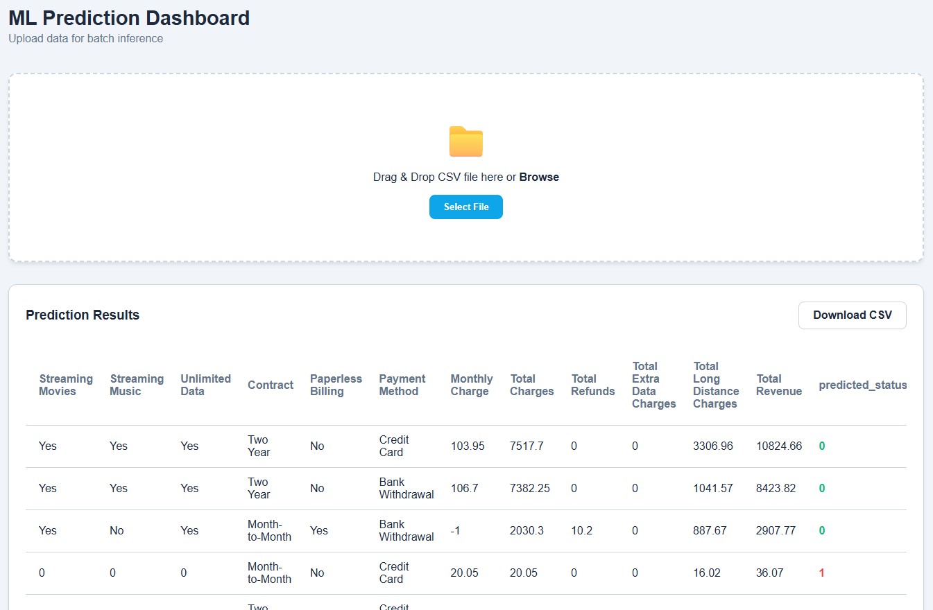
9 Production Deployment & User Interface
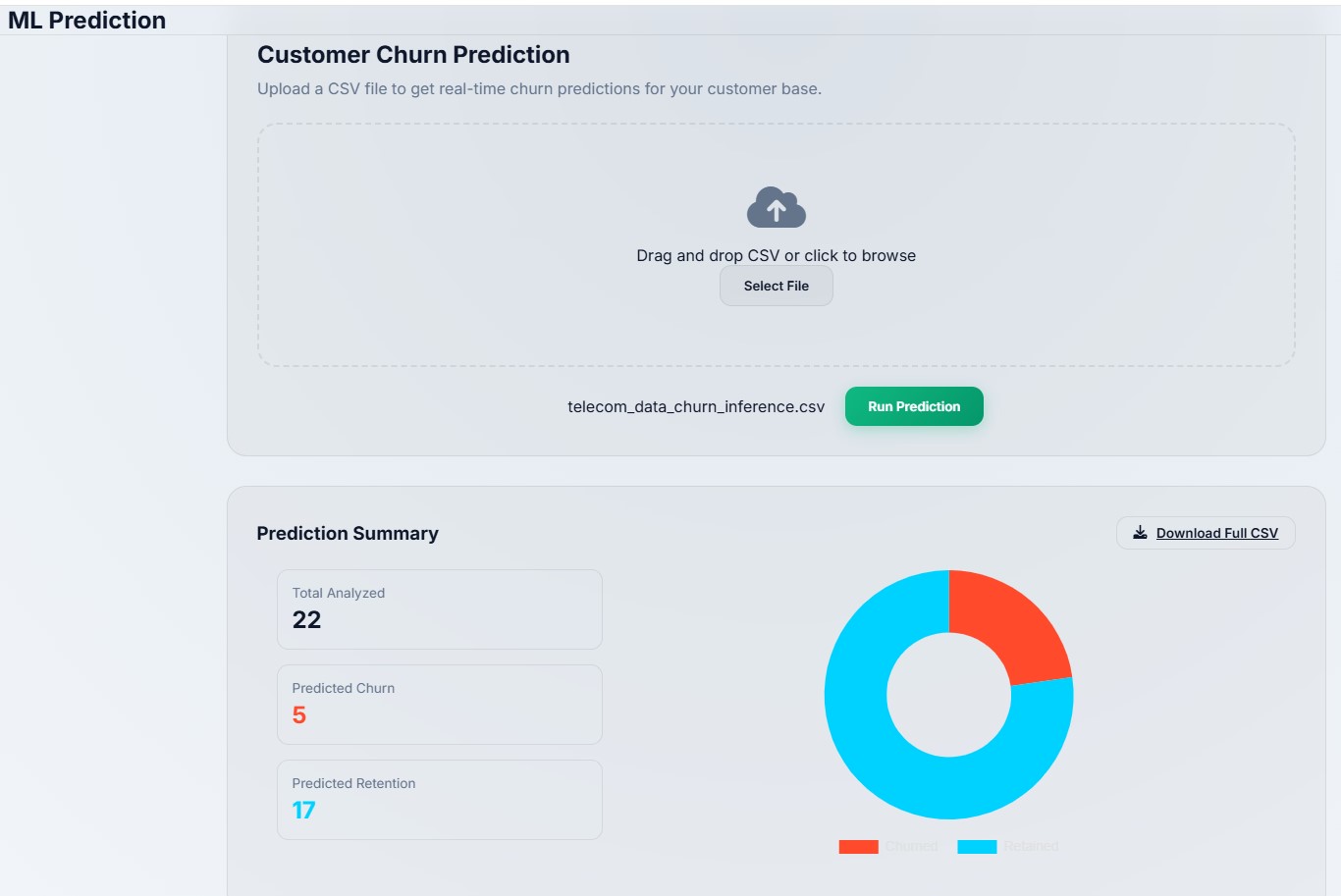
10 Live Demo & Access
A live deployed version of the system is available at:
Contact me to request the inference data.
11 Bonus
- Balancing bias–variance trade-offs:
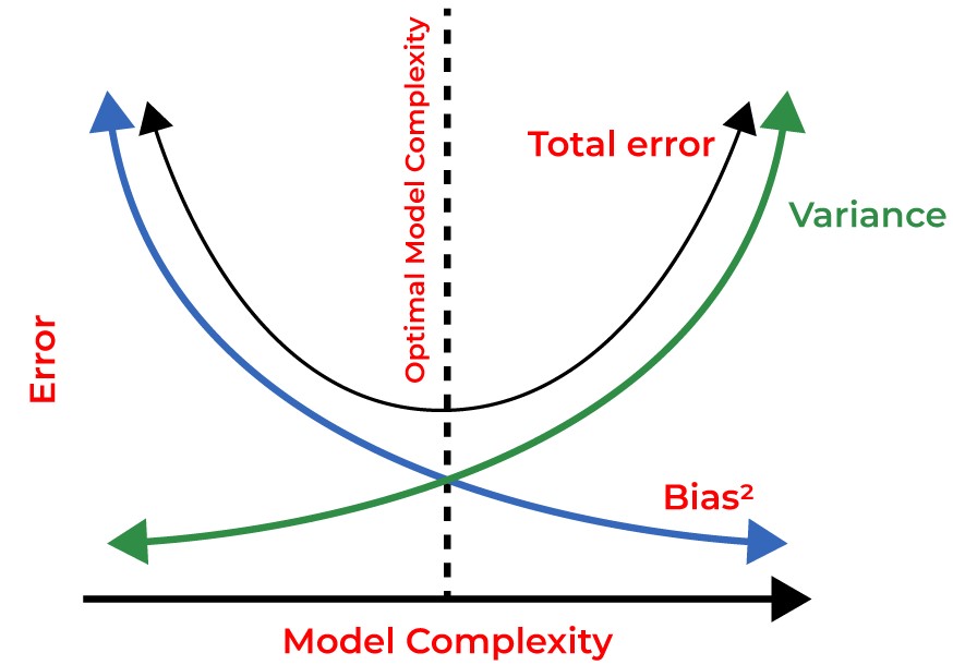
The bias-variance tradeoff is the fundamental principle that you cannot simultaneously minimize both bias and variance. As you make your model more complex to reduce bias (better fit to training data), you inevitably increase variance (sensitivity to training data changes). The goal is finding the optimal balance where total error is minimized. This tradeoff is crucial because it guides every major decision in model selection, from choosing algorithms to tuning hyperparameters.
* High bias: Underfitting (poor performance on both training and validation data, with training and validation errors that are similar but both unacceptably high)
* High variance: Overfitting (good performance on training data but poor performance on validation data, with training error being low but validation error being high)
High bias manifests as poor performance on both training and test datasets, with similar error levels on both. Your model consistently underperforms because it’s too simple to capture the underlying patterns. High variance shows excellent training performance but poor test performance (a large gap between training and validation errors). You can diagnose these issues using learning curves, cross-validation results, and comparing training versus validation metrics.
High bias algorithms include linear regression, logistic regression, and Naive Bayes - they make strong assumptions about data relationships. High variance algorithms include deep decision trees, k-nearest neighbors with low k values, and complex neural networks - they can model intricate patterns but are sensitive to training data changes. Balanced algorithms like Support Vector Machines and Random Forest (through ensemble averaging) manage both bias and variance more effectively.
- Diagnosis of High Bias and High Variance
- You can diagnose these issues using learning curves, cross-validation results, and comparing training versus validation metrics.
- Learning Curves:
- Learning curves show the relationship between model performance and the amount of training data. They can help you identify whether your model is suffering from high bias or high variance.
- High bias manifests as poor performance on both training and test datasets, with similar error levels on both. Your model consistently underperforms because it’s too simple to capture the underlying patterns. High variance shows excellent training performance but poor test performance (a large gap between training and validation errors).
- Learning curves show the relationship between model performance and the amount of training data. They can help you identify whether your model is suffering from high bias or high variance.
- Cross-Validation:
- Follows similar intuitions as learning curves.
- Follows similar intuitions as learning curves.
- Training vs Validation Metrics:
- Also follows similar intuitions as learning curves.
- Also follows similar intuitions as learning curves.
- Learning Curves:
- You can diagnose these issues using learning curves, cross-validation results, and comparing training versus validation metrics.
- Reducing Bias and Variance in Real Models
- Bias:
Use more complex algorithms for example, switching from linear regression to polynomial regression, or from logistic regression to a neural network.
Use more diverse training data for example, collecting more training data or using data from different sources.
Use feature engineering for example, creating new features or selecting relevant features.
Remove regularization constraints that might be oversimplifying your model.
- Variance:
Add regularization constraints that prevent the model from fitting noise for example;
- L1 regularization (Lasso) can drive some coefficients to zero, effectively performing feature selection, which increases bias slightly but reduces variance significantly.
- L2 regularization (Ridge) can shrink coefficients but not drive them to zero, which can help reduce variance while maintaining some model complexity.
- ElasticNet combines L1 and L2 regularization, offering a balance between feature selection and coefficient shrinkage.
- Dropout in neural networks randomly deactivates units during training, which helps prevent overfitting by forcing the network to learn more robust features.
- Early stopping monitors validation performance and stops training when performance starts to degrade, preventing overfitting.
- Data augmentation artificially increases the size of your training dataset by generating variations of your existing data.
- Batch normalization standardizes input features, which can help prevent overfitting by making the model less sensitive to specific input values.
- L1 regularization (Lasso) can drive some coefficients to zero, effectively performing feature selection, which increases bias slightly but reduces variance significantly.
Cross-validation becomes crucial for variance reduction because it gives a more reliable estimate of your model’s true performance.
Use simpler algorithms for example, switching from a neural network to linear regression.
Use feature selection (for example, selecting relevant features).
- Bias: